Chi-square test of independence in R

Test whether two categorical variables are associated using the chi-square test in R — building the contingency table, running chisq.test, and knowing when to switch to Fisher’s exact test.

When both of your variables are categorical, the chi-square test of independence asks: are they associated, or independent? Here’s the full workflow in R. (Unsure this is the right test? Check the which-test tool.)

Build the contingency table

We’ll use the built-in HairEyeColor data, collapsed to a hair-colour × eye-colour table:

tab <- apply(HairEyeColor, c(1, 2), sum)
tab

       Eye
Hair    Brown Blue Hazel Green
  Black    68   20    15     5
  Brown   119   84    54    29
  Red      26   17    14    14
  Blond     7   94    10    16

Run the test

chisq.test(tab)

    Pearson's Chi-squared test

data:  tab
X-squared = 138.29, df = 9, p-value < 2.2e-16

A small p-value means hair colour and eye colour are not independent — there’s an association. The test compares the observed counts to the counts you’d expect if the two variables were unrelated.

mosaicplot(tab, color = c("#1b2a4a", "#2f6fed", "#17a2b8", "#5aa0ff"),
           main = "Hair vs eye colour", las = 1)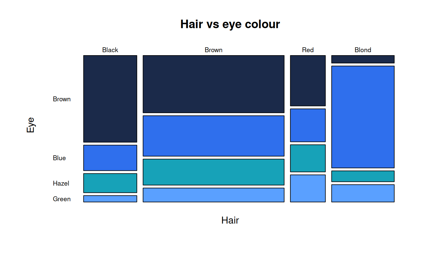

Figure 1

The mosaic plot makes the association visible — tile areas are proportional to counts, and the pattern departs clearly from a plain grid.

When to use Fisher’s exact test instead

The chi-square approximation gets unreliable when expected cell counts are small (a common rule: any expected count < 5). R even warns you. In that case, use the exact alternative:

fisher.test(matrix(c(8, 2, 1, 9), nrow = 2))

    Fisher's Exact Test for Count Data

data:  matrix(c(8, 2, 1, 9), nrow = 2)
p-value = 0.005477
alternative hypothesis: true odds ratio is not equal to 1
95 percent confidence interval:
    2.057999 1740.081669
sample estimates:
odds ratio 
  27.32632 

Check expected counts with chisq.test(tab)$expected, and switch to fisher.test() for small tables.

Reporting it

Report the statistic, degrees of freedom, p-value and — crucially — an effect size such as Cramér’s V, since a large sample can make a trivial association “significant.”

---

Categorical data with more structure than a single table? That’s where we come in.