Publication-quality Kaplan–Meier curves with survival + ggplot2

The survfit object has everything you need; ggplot2 does the rest. A dependency-light recipe for survival curves you control completely.

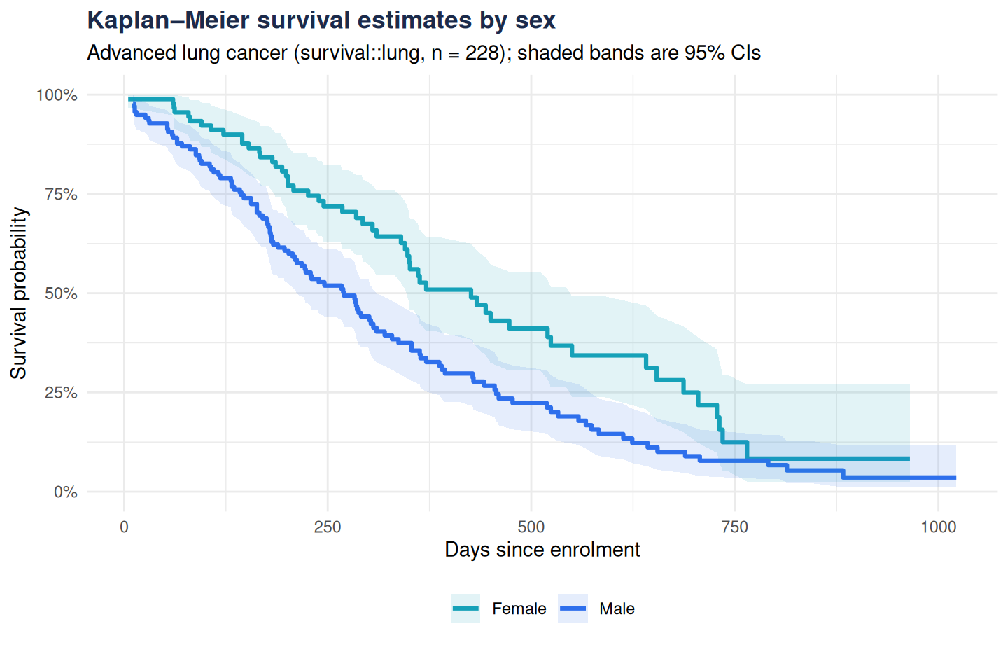
Dedicated packages for plotting survival curves come and go, but the underlying recipe is stable: fit with survival::survfit(), pull the step function out of the object, draw it with ggplot2. Fewer dependencies, full control over every visual detail.

Fit the model

We use the classic lung dataset shipped with the survival package — 228 patients with advanced lung cancer, compared here by sex:

library(survival)

fit <- survfit(Surv(time, status) ~ sex, data = lung)
fit

Call: survfit(formula = Surv(time, status) ~ sex, data = lung)

        n events median 0.95LCL 0.95UCL
sex=1 138    112    270     212     310
sex=2  90     53    426     348     550

Extract the step function

Everything plot(fit) would draw lives inside the object:

km <- data.frame(
  time   = fit$time,
  surv   = fit$surv,
  lower  = fit$lower,
  upper  = fit$upper,
  group  = rep(c("Male", "Female"), times = fit$strata)
)
head(km, 3)

  time      surv     lower     upper group
1   11 0.9782609 0.9542301 1.0000000  Male
2   12 0.9710145 0.9434235 0.9994124  Male
3   13 0.9565217 0.9230952 0.9911586  Male

Draw it

library(ggplot2)

ggplot(km, aes(time, surv, colour = group, fill = group)) +
  geom_step(linewidth = 1.1) +
  geom_ribbon(aes(ymin = lower, ymax = upper),
              stat = "identity", alpha = 0.12, colour = NA) +
  scale_colour_manual(values = c(Male = "#2f6fed", Female = "#17a2b8")) +
  scale_fill_manual(values = c(Male = "#2f6fed", Female = "#17a2b8")) +
  scale_y_continuous(labels = scales::percent, limits = c(0, 1)) +
  labs(
    title = "Kaplan–Meier survival estimates by sex",
    subtitle = "Advanced lung cancer (survival::lung, n = 228); shaded bands are 95% CIs",
    x = "Days since enrolment", y = "Survival probability",
    colour = NULL, fill = NULL
  ) +
  theme_minimal() +
  theme(legend.position = "bottom",
        plot.title = element_text(face = "bold", colour = "#1b2a4a"))

Figure 1

And the test to go with it

A figure without a test is only half the result. The log-rank test:

survdiff(Surv(time, status) ~ sex, data = lung)

Call:
survdiff(formula = Surv(time, status) ~ sex, data = lung)

        N Observed Expected (O-E)^2/E (O-E)^2/V
sex=1 138      112     91.6      4.55      10.3
sex=2  90       53     73.4      5.68      10.3

 Chisq= 10.3  on 1 degrees of freedom, p= 0.001 

The group difference is statistically significant — and because we built the plot ourselves, adding risk tables, median-survival annotations or landmark lines later is just more ggplot2, not a fight with someone else’s defaults.