Repeated-measures ANOVA in R

How to run a repeated-measures ANOVA in R with aov() and an Error() term — the right way to compare three or more measurements on the same subjects — with a trajectory plot.

When you measure the same subjects several times — three time points, three conditions — a plain ANOVA is wrong: it ignores that measurements within a subject are correlated. Repeated-measures ANOVA accounts for that. Here’s the R. (For independent groups, the ANOVA calculator is enough.)

Simulate a within-subject study

Twenty subjects, each measured under three conditions, with real between-subject differences:

set.seed(11)
n <- 20
subj <- factor(rep(1:n, each = 3))
cond <- factor(rep(c("t1", "t2", "t3"), times = n))
b_subj <- rnorm(n, 0, 5)[as.integer(subj)]                 # subject baselines
eff <- c(t1 = 0, t2 = 2, t3 = 4)[as.character(cond)]       # condition effect
y <- 20 + b_subj + eff + rnorm(3 * n, 0, 2)
d <- data.frame(subj, cond, y)

The key: an Error() term

The Error(subj/cond) term tells R that conditions are nested within subjects — this is what makes it repeated-measures rather than a between-groups ANOVA:

summary(aov(y ~ cond + Error(subj / cond), data = d))

Error: subj
          Df Sum Sq Mean Sq F value Pr(>F)
Residuals 19  951.2   50.06               

Error: subj:cond
          Df Sum Sq Mean Sq F value   Pr(>F)    
cond       2  121.3   60.63   19.29 1.65e-06 ***
Residuals 38  119.5    3.14                     
---
Signif. codes:  0 '***' 0.001 '**' 0.01 '*' 0.05 '.' 0.1 ' ' 1

The condition effect is tested against within-subject error, which is smaller because each subject is their own control — so repeated-measures designs are more powerful than between-subject ones.

Plot the trajectories

library(ggplot2)
ggplot(d, aes(cond, y, group = subj)) +
  geom_line(colour = "#8a93a6", alpha = 0.5) +
  stat_summary(aes(group = 1), fun = mean, geom = "line",
               colour = "#2f6fed", linewidth = 1.4) +
  stat_summary(aes(group = 1), fun = mean, geom = "point",
               colour = "#2f6fed", size = 3) +
  labs(title = "Each grey line is a subject; blue is the mean",
       x = "Condition", y = "Outcome") +
  theme_minimal(base_family = "sans") +
  theme(plot.title = element_text(face = "bold", colour = "#1b2a4a"))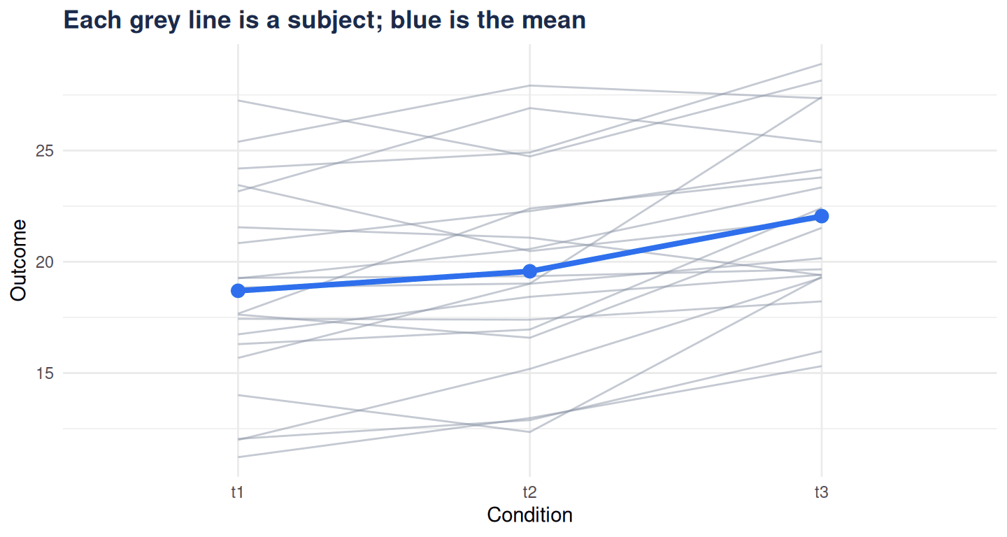

Figure 1

Assumptions and alternatives

Repeated-measures ANOVA assumes sphericity (equal variances of the differences between conditions); when it’s violated, apply a Greenhouse–Geisser correction. For unbalanced data, missing values or more complex designs, a linear mixed model (lme4::lmer) is the modern, more flexible choice — often what we reach for in practice.

---

Longitudinal and repeated-measures designs are easy to get wrong. We handle them properly.