Two-way ANOVA in R

Run and interpret a two-way ANOVA in R with aov() — two factors plus their interaction — using the built-in ToothGrowth data, with an interaction plot.

A one-way ANOVA compares groups on a single factor. A two-way ANOVA brings in a second factor and, crucially, their interaction — does the effect of one factor depend on the other? Here it is in R. (Comparing groups on one factor? Try the ANOVA calculator.)

The data

The built-in ToothGrowth data records tooth length in guinea pigs by supplement type (supp: OJ or VC) and dose (0.5, 1, 2 mg):

ToothGrowth$dose <- factor(ToothGrowth$dose)
fit <- aov(len ~ supp * dose, data = ToothGrowth)
summary(fit)

            Df Sum Sq Mean Sq F value   Pr(>F)    
supp         1  205.4   205.4  15.572 0.000231 ***
dose         2 2426.4  1213.2  92.000  < 2e-16 ***
supp:dose    2  108.3    54.2   4.107 0.021860 *  
Residuals   54  712.1    13.2                     
---
Signif. codes:  0 '***' 0.001 '**' 0.01 '*' 0.05 '.' 0.1 ' ' 1

Reading the three lines

• supp — the main effect of supplement type (averaged over dose).
• dose — the main effect of dose (averaged over supplement).
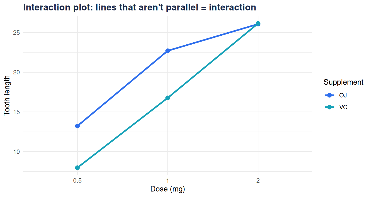
• supp:dose — the interaction: does the supplement effect change with dose? A significant interaction is often the most interesting result — and it means you should interpret the main effects with care.

See the interaction

library(ggplot2)
ggplot(ToothGrowth, aes(dose, len, colour = supp, group = supp)) +
  stat_summary(fun = mean, geom = "line", linewidth = 1.1) +
  stat_summary(fun = mean, geom = "point", size = 2.5) +
  scale_colour_manual(values = c(OJ = "#2f6fed", VC = "#17a2b8")) +
  labs(title = "Interaction plot: lines that aren't parallel = interaction",
       x = "Dose (mg)", y = "Tooth length", colour = "Supplement") +
  theme_minimal(base_family = "sans") +
  theme(plot.title = element_text(face = "bold", colour = "#1b2a4a"))

Figure 1

Non-parallel lines signal an interaction: here the supplement gap is large at low doses and shrinks at the highest dose.

After a significant result

Follow up with post-hoc comparisons that control for multiple testing:

TukeyHSD(fit, "supp")

  Tukey multiple comparisons of means
    95% family-wise confidence level

Fit: aov(formula = len ~ supp * dose, data = ToothGrowth)

$supp
      diff       lwr       upr     p adj
VC-OJ -3.7 -5.579828 -1.820172 0.0002312

And check the usual ANOVA assumptions — roughly normal residuals and similar variances (plot(fit)); see checking normality in R.

---

Factorial designs get subtle fast. When you need them analysed and written up properly, we can help.