set.seed(1)
p_null <- replicate(5000, t.test(rnorm(30), rnorm(30))$p.value)
mean(p_null < 0.05)   # ≈ 0.05 — the Type I error rate
[1] 0.0488Every hypothesis test can be wrong in two ways. Confusing them is one of the most common statistics mistakes — so let’s pin them down and see them in R.
| H₀ true (no effect) | H₀ false (real effect) | |
|---|---|---|
| Reject H₀ | Type I error (false positive), rate = α | Correct (power = 1 − β) |
| Don’t reject | Correct | Type II error (false negative), rate = β |
Under the null, about α of tests are “significant” by chance. Simulate 5,000 tests on data with no real difference:
set.seed(1)
p_null <- replicate(5000, t.test(rnorm(30), rnorm(30))$p.value)
mean(p_null < 0.05) # ≈ 0.05 — the Type I error rate[1] 0.0488Right around 5% — exactly the false-positive rate we chose.
Now give the groups a real difference (d = 0.5) but keep the sample small:
library(ggplot2)
set.seed(2)
sig <- replicate(5000, t.test(rnorm(30), rnorm(30, 0.5))$p.value < 0.05)
power <- mean(sig)

ggplot(data.frame(x = c("Missed (Type II)", "Detected"),
                  y = c(1 - power, power)),
       aes(x, y, fill = x)) +
  geom_col(width = 0.6, show.legend = FALSE) +
  scale_fill_manual(values = c("Detected" = "#2f6fed", "Missed (Type II)" = "#b02a37")) +
  scale_y_continuous(labels = scales::percent) +
  labs(title = sprintf("Real effect (d=0.5), n=30: power = %.0f%%", power * 100),
       x = NULL, y = NULL) +
  theme_minimal(base_family = "sans") +
  theme(plot.title = element_text(face = "bold", colour = "#1b2a4a"))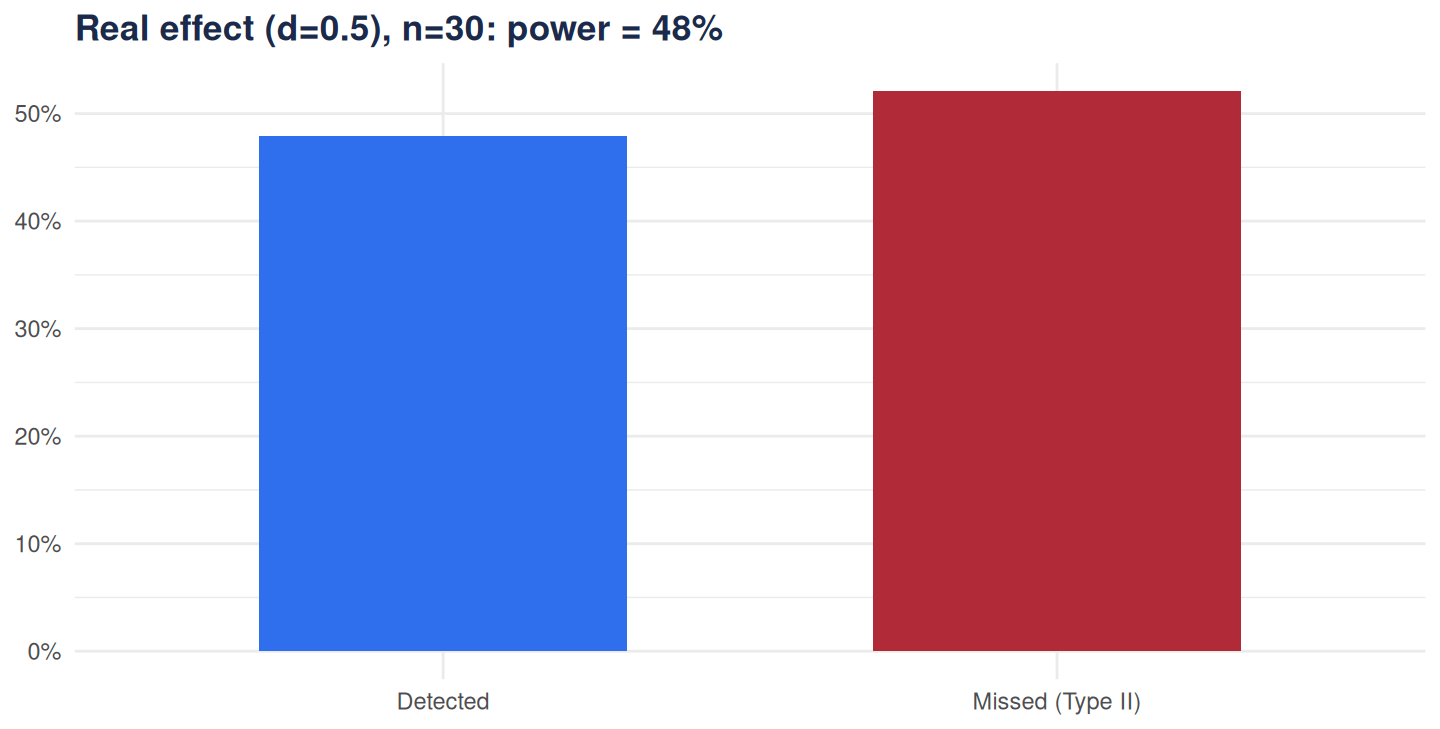
A real effect, yet a big chunk of tests miss it — that’s Type II error from being underpowered.
You can’t drive both errors to zero at once. You choose α, and you buy power (lower β) mainly with sample size — which is why a power analysis before data collection matters so much. Plan it with our sample size calculator.
Designing a study so it can actually detect what you care about? We can help.