Z-scores explained (with R): standardising, percentiles and probabilities

What a z-score is, how it maps to a percentile, and how to compute z-scores and normal probabilities in R with pnorm and qnorm — the intuition and the code.

A z-score answers a simple question: how unusual is this value? It rescales any measurement into standard-deviation units so you can compare across different scales and read off a percentile. Here’s the idea and the R. (Just need a number? Use our z-score calculator.)

The definition

\[z = \frac{x - \mu}{\sigma}\]

A z of 0 is exactly average, +1 is one SD above the mean, −2 is two SDs below. Because the standard normal distribution is fixed, each z maps to a percentile — the share of the population below it.

# a value of 130 on a scale with mean 100, SD 15
z <- (130 - 100) / 15
z

[1] 2

pnorm(z)          # percentile: share below 130

[1] 0.9772499

So 130 sits at about the 98th percentile.

See it on the curve

library(ggplot2)
x <- seq(-4, 4, length.out = 400)
d <- data.frame(x, y = dnorm(x))

ggplot(d, aes(x, y)) +
  geom_area(data = subset(d, x <= 2), fill = "#2f6fed", alpha = 0.25) +
  geom_line(colour = "#1b2a4a", linewidth = 1) +
  geom_vline(xintercept = 2, linetype = 2, colour = "#b02a37") +
  annotate("text", x = 0, y = 0.15, label = "97.7%", colour = "#1b2a4a", fontface = "bold") +
  labs(title = "z = 2 sits at the 97.7th percentile",
       x = "z-score", y = "Density") +
  theme_minimal(base_family = "sans") +
  theme(plot.title = element_text(face = "bold", colour = "#1b2a4a"))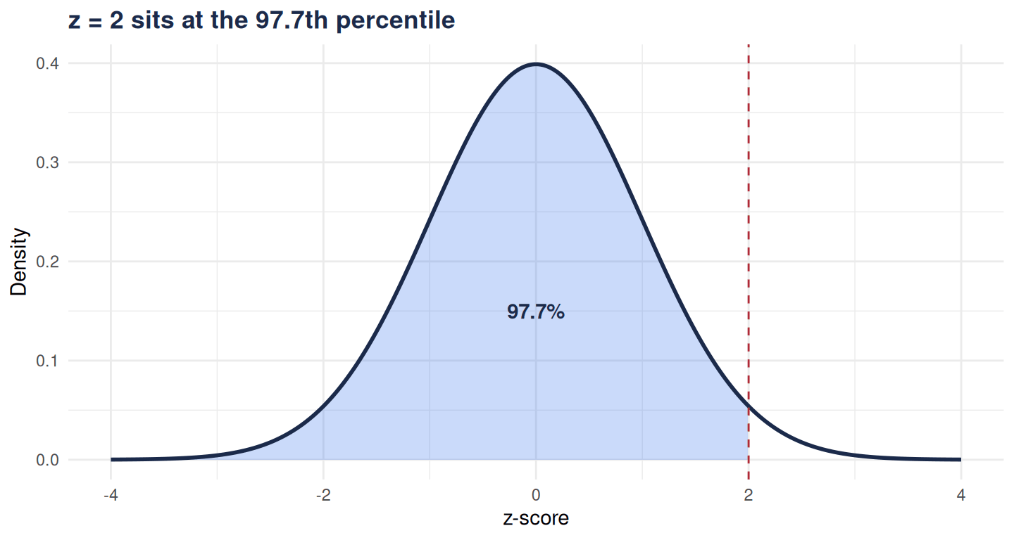

Figure 1

The three moves

pnorm(1.96)        # z-score -> cumulative probability

[1] 0.9750021

qnorm(0.975)       # probability -> z-score

[1] 1.959964

1 - pnorm(2)       # upper tail: share ABOVE a z of 2

[1] 0.02275013

pnorm() goes from z to probability; qnorm() goes back. That’s why ±1.96 brackets the middle 95% — qnorm(0.975) is 1.96.

The one caveat

Standardising assumes an approximately normal distribution, and that you know (or can treat as known) the SD. For small samples where the SD is estimated, use the t-distribution instead — it has heavier tails.

---

Standardising is step one. When you need the whole analysis, that’s our work.