Clinical R Toolkit

clinical

biostatistics

Runnable R recipes for clinical research: a Table 1 with gtsummary, logistic regression with odds ratios and ROC/AUC, Cox proportional hazards with assumption checks, and diagnostic test accuracy — all reproducible.

The analyses we run most often for clinical and health-sciences research, as copy-paste R you can adapt to your own data. Every table and figure below is generated live by R when this page builds — nothing is a screenshot. The examples use the built-in gtsummary::trial clinical-trial dataset and survival::lung, so they run anywhere.

Need one of these applied to your data, with full assumption diagnostics and an APA-ready write-up? That’s our statistical analysis service.

Describe your cohort

1. Table 1 — baseline characteristics

The first table in almost every clinical paper: participant characteristics by group, with the right summary per variable type and a test column. gtsummary does it in a few lines.

library(gtsummary)

trial |>
  dplyr::select(trt, age, grade, stage, marker) |>
  tbl_summary(
    by = trt,
    label = list(age ~ "Age (years)", marker ~ "Marker level (ng/mL)"),
    missing_text = "(missing)"
  ) |>
  add_p() |>
  add_overall() |>
  bold_labels() |>
  modify_caption("**Table 1. Baseline characteristics by treatment arm**")

**Table 1. Baseline characteristics by treatment arm**
Characteristic	Overall N = 200¹	Drug A N = 98¹	Drug B N = 102¹	p-value²
Age (years)	47 (38, 57)	46 (37, 60)	48 (39, 56)	0.7
(missing)	11	7	4
Grade				0.9
I	68 (34%)	35 (36%)	33 (32%)
II	68 (34%)	32 (33%)	36 (35%)
III	64 (32%)	31 (32%)	33 (32%)
T Stage				0.9
T1	53 (27%)	28 (29%)	25 (25%)
T2	54 (27%)	25 (26%)	29 (28%)
T3	43 (22%)	22 (22%)	21 (21%)
T4	50 (25%)	23 (23%)	27 (26%)
Marker level (ng/mL)	0.64 (0.22, 1.41)	0.84 (0.23, 1.60)	0.52 (0.18, 1.21)	0.085
(missing)	10	6	4
¹ Median (Q1, Q3); n (%)
² Wilcoxon rank sum test; Pearson’s Chi-squared test

Continuous variables get median (IQR), categoricals get n (%), the test is chosen automatically, and missing data is counted explicitly rather than silently dropped.

Binary outcomes

2. Logistic regression — odds ratios & ROC/AUC

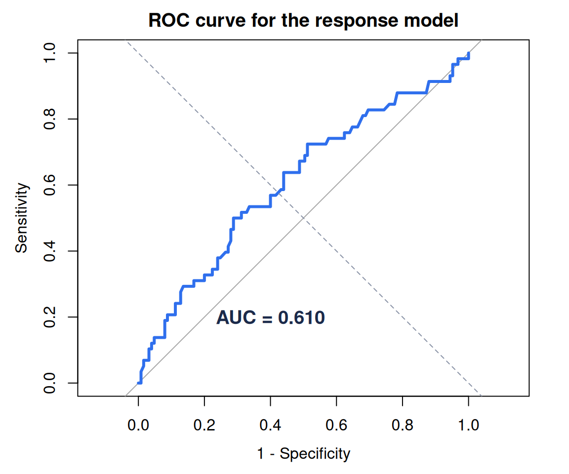
For a binary outcome (here, tumour response), fit a logistic model, report adjusted odds ratios with confidence intervals, then quantify discrimination with the ROC curve and AUC.

library(survival)

d <- na.omit(trial[, c("response", "age", "grade", "stage")])
fit <- glm(response ~ age + grade + stage, data = d, family = binomial)

tbl_regression(fit, exponentiate = TRUE) |>
  bold_p() |>
  modify_caption("**Adjusted odds ratios for tumour response**")

**Adjusted odds ratios for tumour response**
Characteristic	OR	95% CI	p-value
Age	1.02	1.00, 1.04	0.092
Grade
I	—	—
II	0.84	0.38, 1.85	0.7
III	1.05	0.49, 2.25	>0.9
T Stage
T1	—	—
T2	0.57	0.23, 1.34	0.2
T3	0.91	0.37, 2.22	0.8
T4	0.76	0.31, 1.85	0.6
Abbreviations: CI = Confidence Interval, OR = Odds Ratio

library(pROC)

roc_obj <- roc(d$response, fitted(fit), quiet = TRUE)

plot(roc_obj, col = "#2f6fed", lwd = 3, legacy.axes = TRUE,
     xlab = "1 - Specificity", ylab = "Sensitivity",
     main = "ROC curve for the response model")
abline(0, 1, lty = 2, col = "#8a93a6")
text(0.6, 0.2, sprintf("AUC = %.3f", as.numeric(auc(roc_obj))),
     col = "#1b2a4a", font = 2, cex = 1.2)

The odds-ratio table answers “which factors matter, and by how much?”; the AUC answers “how well does the model separate responders from non-responders?”

Time-to-event

3. Cox proportional hazards — with assumption checks

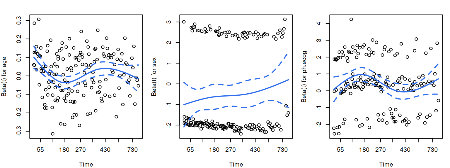
A hazard ratio is only trustworthy if the proportional-hazards assumption holds. Fit the model, report hazard ratios, then test the assumption with cox.zph() — never skip the second step.

cx <- coxph(Surv(time, status) ~ age + sex + ph.ecog, data = lung)

tbl_regression(cx, exponentiate = TRUE,
               label = list(sex ~ "Sex (2 = female)",
                            ph.ecog ~ "ECOG performance score")) |>
  bold_p() |>
  modify_caption("**Hazard ratios, advanced lung cancer (survival::lung)**")

**Hazard ratios, advanced lung cancer (survival::lung)**
Characteristic	HR	95% CI	p-value
age	1.01	0.99, 1.03	0.2
Sex (2 = female)	0.58	0.41, 0.80	<0.001
ECOG performance score	1.59	1.27, 1.99	<0.001
Abbreviations: CI = Confidence Interval, HR = Hazard Ratio

zph <- cox.zph(cx)
zph

        chisq df    p
age     0.188  1 0.66
sex     2.305  1 0.13
ph.ecog 2.054  1 0.15
GLOBAL  4.464  3 0.22

par(mfrow = c(1, 3), mar = c(4, 4, 2, 1), family = "sans")
plot(zph, col = "#2f6fed", lwd = 2)

A non-significant global test (and flat scaled-Schoenfeld residuals) means proportional hazards is a defensible assumption. A small p is a warning, not a verdict — it points you toward stratification, time-varying effects or a different model.

Screening & tests

4. Diagnostic test accuracy

Sensitivity, specificity, predictive values and likelihood ratios from a 2×2 table — the numbers a clinician actually asks for. Base R, no dependencies.

# 2x2 counts: rows = test result, columns = true disease status
tp <- 90; fp <- 10   # test positive: disease present / absent
fn <- 20; tn <- 180  # test negative: disease present / absent

diag_accuracy <- function(tp, fp, fn, tn) {
  sens <- tp / (tp + fn)
  spec <- tn / (tn + fp)
  data.frame(
    Metric = c("Sensitivity", "Specificity",
               "Positive predictive value", "Negative predictive value",
               "Positive likelihood ratio", "Negative likelihood ratio"),
    Estimate = round(c(
      sens, spec,
      tp / (tp + fp), tn / (tn + fn),
      sens / (1 - spec), (1 - sens) / spec
    ), 3)
  )
}

knitr::kable(diag_accuracy(tp, fp, fn, tn))

Metric	Estimate
Sensitivity	0.818
Specificity	0.947
Positive predictive value	0.900
Negative predictive value	0.900
Positive likelihood ratio	15.545
Negative likelihood ratio	0.192

Remember that predictive values depend on prevalence — the same test looks very different in a screening population versus a specialist clinic. When that matters, we model PPV/NPV across the plausible prevalence range (try the diagnostic-test calculator in our live demos).

1. Table 1 — baseline characteristics

2. Logistic regression — odds ratios & ROC/AUC

3. Cox proportional hazards — with assumption checks

4. Diagnostic test accuracy

More in the same vein