Chi-square goodness-of-fit test in R

Use the chi-square goodness-of-fit test in R to check whether observed counts match an expected distribution — is a die fair, do categories match expected proportions — with chisq.test.

The chi-square goodness-of-fit test asks: do my observed category counts match a distribution I expected? Is this die fair? Do these blood types match population proportions? It’s the one-variable cousin of the test of independence. Here it is in R. (Testing two variables in a table instead? Use our chi-square calculator.)

Is the die fair?

Roll a die 120 times. If it’s fair, you’d expect 20 of each face. Here’s what you actually got:

observed <- c(22, 17, 20, 18, 13, 30)   # counts for faces 1–6
chisq.test(observed, p = rep(1/6, 6))

    Chi-squared test for given probabilities

data:  observed
X-squared = 8.3, df = 5, p-value = 0.1405

p = rep(1/6, 6) says “expect equal proportions.” A small p-value would be evidence the die is not fair.

Observed vs expected

library(ggplot2)
d <- data.frame(face = factor(1:6),
                observed = observed,
                expected = sum(observed) / 6)

ggplot(d, aes(face)) +
  geom_col(aes(y = observed), fill = "#2f6fed", width = 0.6) +
  geom_hline(yintercept = d$expected[1], linetype = 2, colour = "#b02a37", linewidth = 1) +
  annotate("text", x = 6.3, y = d$expected[1], label = "expected", colour = "#b02a37", hjust = 0) +
  labs(title = "Observed counts vs the expected 20 per face",
       x = "Die face", y = "Count") +
  coord_cartesian(xlim = c(0.5, 7)) +
  theme_minimal(base_family = "sans") +
  theme(plot.title = element_text(face = "bold", colour = "#1b2a4a"))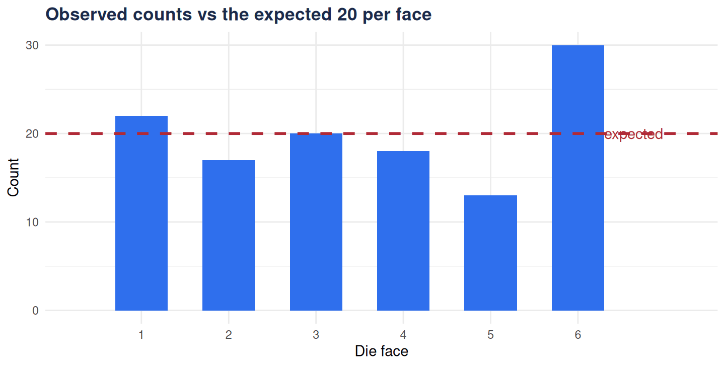

Figure 1

Face 6 came up a lot and face 5 rarely — the test tells you whether that pattern is more than chance.

Testing custom proportions

Goodness-of-fit isn’t limited to “all equal.” Supply any expected proportions — for example, testing whether observed genotype counts match a 1:2:1 ratio:

chisq.test(c(30, 55, 15), p = c(0.25, 0.5, 0.25))

    Chi-squared test for given probabilities

data:  c(30, 55, 15)
X-squared = 5.5, df = 2, p-value = 0.06393

Watch the expected counts

Like all chi-square tests, the approximation needs reasonably large expected counts (a common rule: at least 5 per category). With sparse categories, collapse them or use an exact/simulation-based test (chisq.test(..., simulate.p.value = TRUE)).

---

Categorical data with more structure than one table? That’s where we come in.