Clinical trial tables, listings and figures produced in R — demography Table 1, adverse-event summary, lab shift table, Kaplan-Meier curve and subgroup forest plot, each shown against its mock shell.
Every clinical deliverable starts as a mock shell and ends as a table or figure that must match it to the cell. Below are five standard CSR outputs, each shown as shell → R output. Everything on this page is produced live by R when the page is built — the code is the deliverable.
Data note: outputs use the gtsummary::trial teaching dataset and small synthetic ADaM-style datasets generated on this page — structures are CDISC-shaped, values are fictional.
1. Demography — Table 1
Shell:
Table 14.1.1  Demographic and Baseline Characteristics — ITT Population
                        Drug A          Drug B          Total
                        (N = xx)        (N = xx)        (N = xx)
Age, years
  Mean (SD)             xx.x (xx.x)     xx.x (xx.x)     xx.x (xx.x)
Grade, n (%)
  I / II / III          xx (xx.x) ...
Table 14.3.1  Adverse Events by System Organ Class and Preferred Term — Safety Population
                                    Drug A (N = xx)    Placebo (N = xx)
System Organ Class
  Patients with >=1 event           xx (xx.x%)         xx (xx.x%)
    Preferred term                  xx                 xx
R output (rtables + tern):
library(rtables)library(tern) # clinical analyze functions on top of rtableslibrary(dplyr)set.seed(2026)adsl <-tibble(USUBJID =sprintf("01-%03d", 1:80),ARM =rep(c("Drug A", "Placebo"), each =40))adae <-tibble(USUBJID =sample(adsl$USUBJID, 120, replace =TRUE),AESOC =sample(c("Gastrointestinal disorders", "Nervous system disorders","Infections and infestations"), 120, replace =TRUE,prob =c(.4, .35, .25)),AEDECOD =sample(c("Nausea", "Diarrhoea", "Headache", "Dizziness","Nasopharyngitis"), 120, replace =TRUE)) |>left_join(adsl, by ="USUBJID")basic_table(show_colcounts =TRUE) |>split_cols_by("ARM") |>split_rows_by("AESOC", split_fun = drop_split_levels) |>summarize_num_patients(var ="USUBJID", .stats ="unique",.labels =c(unique ="Patients with >=1 event")) |>count_occurrences(vars ="AEDECOD") |>build_table(adae, alt_counts_df = adsl)
Warning: Non-unique sibling analysis table names. Using Labels instead. Use the table_names argument to analyze to avoid this when analyzing the same variable multiple times.
    occured at (row) path: BASE[Normal]
Warning: Non-unique sibling analysis table names. Using Labels instead. Use the table_names argument to analyze to avoid this when analyzing the same variable multiple times.
    occured at (row) path: BASE[High]
                   Drug A        Placebo
Baseline ALT       (N=40)        (N=40)
——————————————————————————————————————————
Normal
  Post: Normal   29 (87.88%)   27 (75.00%)
  Post: High     4 (12.12%)    9 (25.00%)
High
  Post: Normal   5 (71.43%)    3 (75.00%)
  Post: High     2 (28.57%)    1 (25.00%)
4. Kaplan-Meier figure
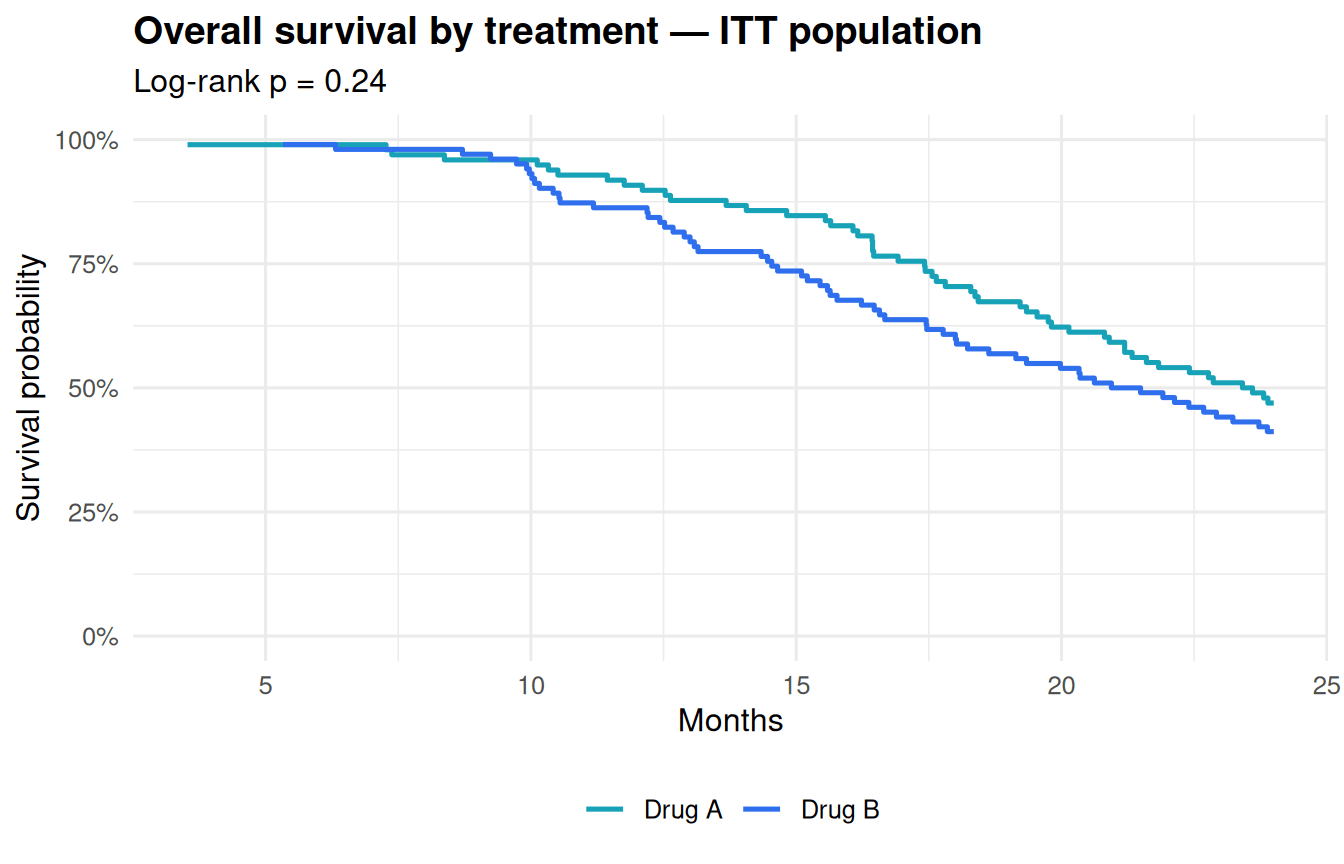
Shell:Figure 14.2.1 — Kaplan-Meier plot of overall survival by treatment, ITT population; number at risk below the x-axis; log-rank p in the panel.
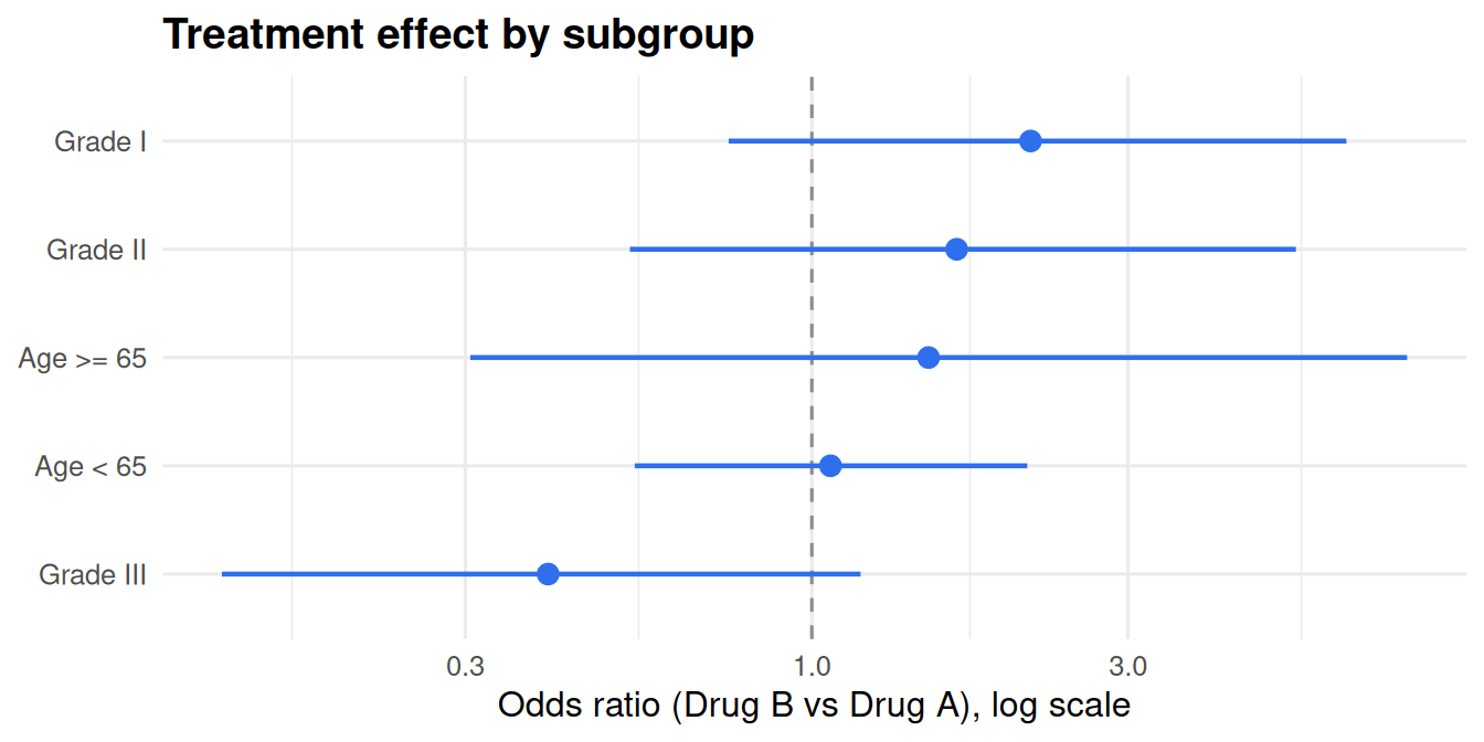
Shell:Figure 14.2.4 — Treatment effect (odds ratio, 95% CI) by subgroup; reference line at OR = 1.
R output:
library(dplyr)subgroups <-bind_rows( trial |>mutate(sub =ifelse(age <65, "Age < 65", "Age >= 65")), trial |>mutate(sub =paste("Grade", grade))) |>filter(!is.na(sub), !is.na(age)) |>group_by(sub) |>group_modify(~ { m <-glm(response ~ trt, family = binomial, data = .x) ci <-suppressMessages(confint(m))data.frame(or =exp(coef(m)[2]), lo =exp(ci[2, 1]), hi =exp(ci[2, 2])) }) |>ungroup()ggplot(subgroups, aes(or, reorder(sub, or))) +geom_vline(xintercept =1, linetype =2, colour ="grey55") +geom_pointrange(aes(xmin = lo, xmax = hi), colour ="#2f6fed", linewidth =0.8) +scale_x_log10() +labs(x ="Odds ratio (Drug B vs Drug A), log scale", y =NULL,title ="Treatment effect by subgroup") +theme_minimal(base_size =12) +theme(plot.title =element_text(face ="bold"))
How these become deliverables
Each output exports to the format your shell demands — as_flex_table() to Word for gtsummary, export_as_rtf() for rtables, ggsave() at journal DPI for figures — inside a parameterised Quarto pipeline that regenerates the whole TLF package from the analysis datasets in one run. The datasets themselves are derived with admiral, and the QC side is double programming.
Have a shell package waiting?
Send us two or three representative shells and we’ll quote the whole package — fixed price, double-programmed. Contact us →
Free R, Markdown & Quarto cheat sheets
One-page PDF guides — the “Which test?” decision chart, Markdown syntax, and Quarto reporting — free to download. Add your email for the occasional R tip too. No spam, unsubscribe anytime.