library(gtsummary)

d <- na.omit(trial[, c("response", "age", "marker", "stage")])
fit <- glm(response ~ age + marker + stage, data = d, family = binomial)Logistic regression in R: odds ratios and ROC/AUC, done right
clinical
biostatistics
regression
pROC
A binary clinical outcome needs two things: adjusted odds ratios that answer ‘what matters?’ and an ROC/AUC that answers ‘how well does the model discriminate?’. Here is the clean R workflow for both.
For a yes/no clinical outcome — responded or not, readmitted or not — logistic regression is the workhorse. But a model isn’t finished at the coefficient table. You need adjusted odds ratios to interpret effects and a ROC curve with AUC to judge how well the model actually separates the two groups.
Fit the model
Using the trial dataset (response = tumour response), we adjust for age, marker level and disease stage. Fit on complete cases so the model and the ROC use the same rows:
Odds ratios that read cleanly
tbl_regression(exponentiate = TRUE) turns the raw log-odds coefficients into odds ratios with confidence intervals and p-values — the format a journal expects:
tbl_regression(fit, exponentiate = TRUE) |>
  bold_p() |>
modify_caption("**Adjusted odds ratios for tumour response**")| Characteristic | OR | 95% CI | p-value |
|---|---|---|---|
| Age | 1.02 | 1.00, 1.04 | 0.11 |
| Marker Level (ng/mL) | 1.38 | 0.95, 2.03 | 0.092 |
| T Stage | |||
| T1 | — | — | |
| T2 | 0.46 | 0.18, 1.13 | 0.094 |
| T3 | 0.87 | 0.34, 2.21 | 0.8 |
| T4 | 0.65 | 0.26, 1.62 | 0.4 |
| Abbreviations: CI = Confidence Interval, OR = Odds Ratio | |||
An odds ratio above 1 raises the odds of response, below 1 lowers them; the confidence interval tells you how sure you can be. Because these are adjusted, each is the effect of that variable holding the others fixed.
How well does it discriminate?
Significant predictors don’t guarantee a useful model. The ROC curve plots sensitivity against 1 − specificity across every threshold, and the area under it (AUC) summarises discrimination in a single number — 0.5 is a coin flip, 1.0 is perfect:
library(pROC)

roc_obj <- roc(d$response, fitted(fit), quiet = TRUE)

plot(roc_obj, col = "#2f6fed", lwd = 3, legacy.axes = TRUE,
     xlab = "1 - Specificity", ylab = "Sensitivity",
     main = "ROC curve")
abline(0, 1, lty = 2, col = "#8a93a6")
text(0.6, 0.2, sprintf("AUC = %.3f", as.numeric(auc(roc_obj))),
     col = "#1b2a4a", font = 2, cex = 1.3)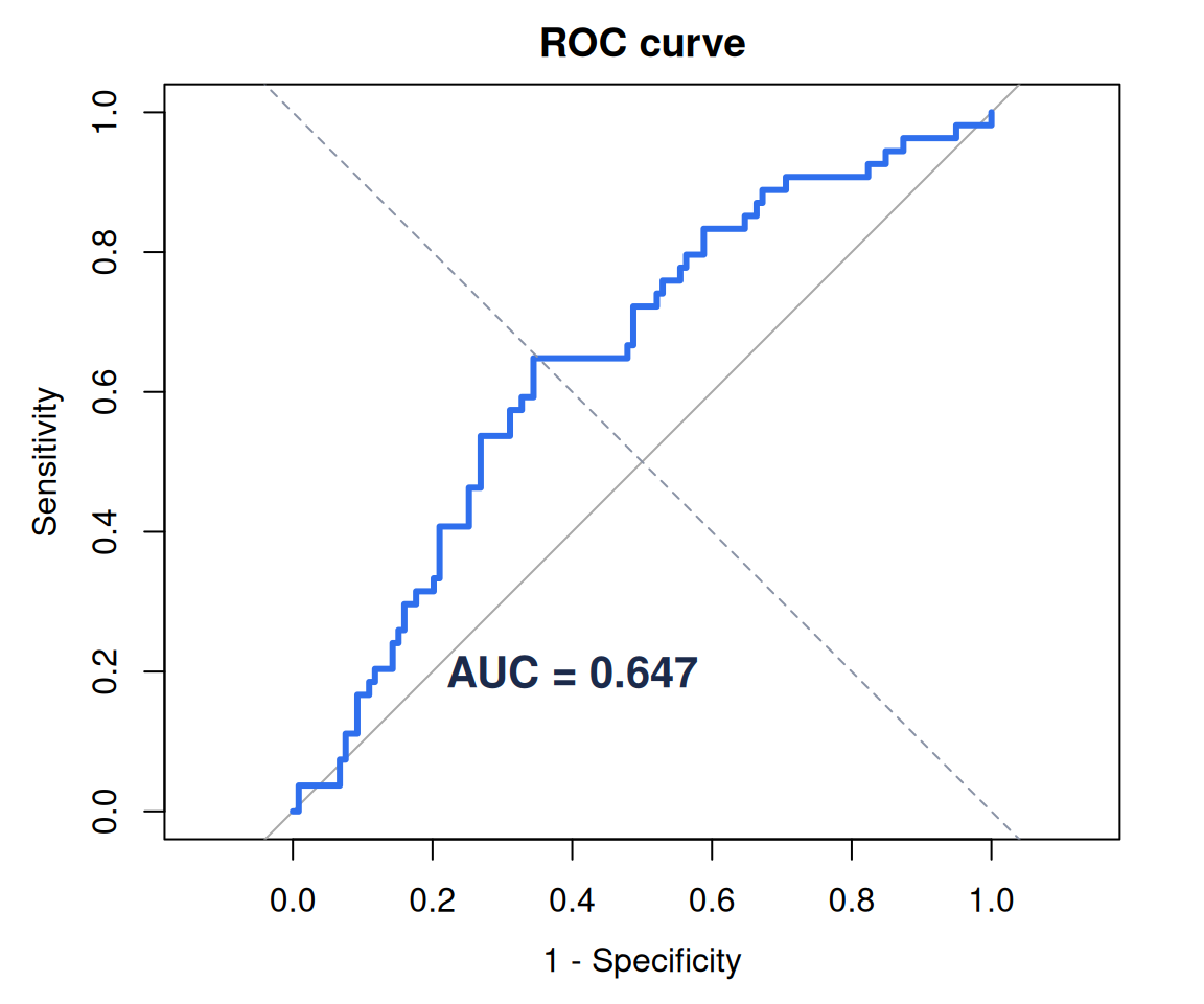
Report the AUC with a confidence interval (ci.auc(roc_obj)) and, if the model will guide decisions, calibration too — discrimination and calibration answer different questions.
The takeaway
Odds ratios tell you which factors matter and by how much; the AUC tells you whether the model is worth using at all. A complete logistic analysis reports both — and, ideally, is reproducible from raw data to figure in one script.
See this alongside survival and diagnostic-test recipes in our Clinical R toolkit.
Part of our guide to biostatistics in R.